The essence of time-nuttery is measuring the stability of clocks and oscillators. Allan Deviation (“ADEV”) is the statistic most commonly used to talk about frequency stability. There’s a very good article about it on Wikipedia, but it’s a bit deep for many. This post is a TL;DR description. To keep it simple I’m skipping over a lot and making analogies that may not quite be correct (fellow time-nuts, please forgive me).[1]One simplification is that I’m almost always going to be talking about “deviation” but the underlying statistic is actually variation. Deviation is the square root of the variance. The post at https://www.mathsisfun.com/data/standard-deviation.html does a good job explaining it. But hopefully this will help you understand an ADEV plot without your eyes glazing over.
There is variation from the ideal values in just about any set of data. Standard deviation is a statistic commonly used to understand that variation, or “variance”. It gives you an idea of the how the data is distributed around the mean value. Under the right circumstances it can help predict future results based on past performance. But it only works well for noise that has certain characteristics (“noise” is the generic term for unwanted variance in signals; there are many types).
Unfortunately, oscillator noise does not have those characteristics. Specifically, the results of a standard deviation calculation should converge. In other words, the more data points you have, the more certain the measurement should become.
The types of noise encountered in oscillators, though, does not always converge; sometimes the more data you have, the less reliable the standard deviation calculation becomes. Allan Deviation was created by David Allan as a statistic that does converge with oscillator noise.
The main purpose of ADEV is to quantify the likely difference between any two successive measurements taken a specified time interval apart. Shorthand for that measurement interval is the Greek character tau. I try to avoid jargon in these posts, but “tau” is so much easier than “measurement interval” that I’ll use it frequently.
Often ADEV at a single tau does not tell the full story because the quantity and type of noise changes with the interval between measurements. So rather than a single number, ADEV is usually presented as a plot with tau (time) on the horizontal or X axis, and stability on the vertical or Y axis. Because of the wide range of values on both axes, the plot is usually made in log-log form, so each major tick represents one power of ten greater or lesser than the last.
The tau range of interest depends on the device being measured. For example, a stopwatch should be very stable and repeatable over time scales of seconds. On the other hand, the Clock of the Long Now worries about keeping time for the next 10,000 years. For the stopwatch, ADEV at a tau of 1 second is meaningful. For the Long Now, a tau of centuries or even millennia might be appropriate.
Tau is a pretty simple concept — the time between successive measurements) — but the stability number on the Y axis of an ADEV plot might be a bit more challenging. It’s usually expressed as dimensionless fractional frequency error. TThat’s just a fancy name for a ratio — the difference between the nominal frequency and the measured frequency normalized to 1 Hz. It’s “dimensionless” because the nominal frequency could be 1 microHertz or 10 GigaHertz and the relative stability would be the same (in other words, the noise scales with the signal frequency).
With electronic oscillators, the fractional frequency error is often a very small percentage of the carrier frequency, so it’s common to express ADEV with exponential notation rather than a period followed by a bunch of zeroes. As an example of fractional frequency error, let’s look at a 1 MHz oscillator. If we measure an error of 1000 Hz (1 kHz), that is 1×10⁻³, or 1 part per thousand, or 0.1%. Scaling from there, an error at 1 MHz of:
- 1 Hz is 1×10⁻⁶, which is 1 part per million or 0.0001%
- 0.001 Hz (1 mHz) is 1×10⁻⁹, which is 1 part per billion or 0.0000001%
- 0.000001 Hz (1 uHz) is 1×10-12, which is 1 part per trillion or 0.0000000001%
By the way, unless you’re dealing with exotic parts, most of the ADEV values you see will be in the range of parts per million to parts per trillion.
Here’s an example of an ADEV plot, showing the stability of a cesium atomic frequency standard measured against two reference oscillators: another cesium standard (blue trace), and a high-quality crystal oscillator (violet trace):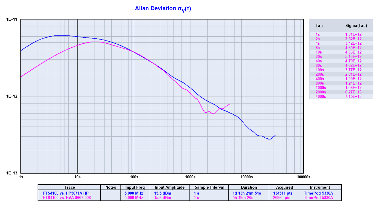
The horizontal axis runs from tau = 1 second to tau = 100000 seconds , with each major line being 10 times the last. The vertical axis runs from 1×10-11 at the top to 1×10-13 at the bottom, again with each line being ten times lower than the last. Lower on the Y axis means less noise, which is a good thing.
Let’s find the ADEV at tau= 100 seconds. Look on the horizontal axis for “100s” and then up from there to where the two traces cross that point, at a bit less than 4×10-12 on the vertical axis. That means that if we take successive measurements 100 seconds apart, it’s likely that their values will be within 4×10-12 of each other.
The right ends of the traces have some strange squiggles and hook upward. It’s a good idea not to trust the last few points on the plot as their potential error is quite high. That’s because it requires at least three measurements at a given tau to calculate the ADEV, and with only three measurements the confidence level is very low. For a given measurement length, there will be fewer data points at long measurement intervals than at short ones. We can have more confidence in ADEV at shorter taus because we have more (or many more) data points; the ADEV converges.
What makes the ADEV graph so useful is that one plot can show an oscillator’s performance over a very wide range of measurement intervals and stability. You get a broad picture in one image.
Another reason that an ADEV plot is useful is that the slope of the plot can indicate the type of noise that predominates at each range of tau. Oscillators can have several types of noise — white noise, random walk noise, flicker noise, and variations of those. An ADEV plot can identify some of these types by their characteristic slope, while other related measurements like Modified Allan Deviation (“MDEV”) can pull out further information. If you’re interested in oscillator noise, this NIST paper is a good (if mathematical) place to start.
MDEV is useful because it can distinguish white noise from flicker noise, if you’re interested in that sort of thing. The Hadamard Deviation (“HDEV”) is interesting because it is not sensitive to frequency drift, which makes it easier to see the underlying performance of some oscillator types that are known to drift even though they are of very high quality — Rubidium vapor and Hydrogen maser standards are in that category. There are also a couple of statistics, Time Deviation (“TDEV”) and Maximum Time Interval Error (“MTIE”) are related statistics that focus more on time rather than frequency performance.
This has been a high level introduction to ADEV. I highly recommend using the Wikipedia article linked above as a starting point if you would like to learn more.
References
| ↑1 | One simplification is that I’m almost always going to be talking about “deviation” but the underlying statistic is actually variation. Deviation is the square root of the variance. The post at https://www.mathsisfun.com/data/standard-deviation.html does a good job explaining it. |
|---|
4 comments
[…] is an Allan Deviation plot of the three […]
[…] For stability analysis, the statistic that is most commonly used is the Allan Deviation. I put up a post describing Allan Deviation that might be interesting and/or useful to […]
[…] Allan Deviation (or ADEV) is a statistic that’s almost universally used in the time and frequency measurement world. It’s very handy for understanding the stability of clocks[1]or oscillators; we tend to think of them as the same thing jQuery('#footnote_plugin_tooltip_891_1_1').tooltip({ tip: '#footnote_plugin_tooltip_text_891_1_1', tipClass: 'footnote_tooltip', effect: 'fade', predelay: 0, fadeInSpeed: 200, delay: 400, fadeOutSpeed: 200, position: 'top center', relative: true, offset: [-7, 0], }); because in a single graph it can span from very short to very long measurement intervals, and from very small to very large amounts of instability, or noise.[2]That huge range is mainly because ADEV plots are almost always log/log, or logarthimic, in both axes. It turns out that’s the best match for typical clock performance curves. jQuery('#footnote_plugin_tooltip_891_1_2').tooltip({ tip: '#footnote_plugin_tooltip_text_891_1_2', tipClass: 'footnote_tooltip', effect: 'fade', predelay: 0, fadeInSpeed: 200, delay: 400, fadeOutSpeed: 200, position: 'top center', relative: true, offset: [-7, 0], }); I’ll be using it a lot because ADEV allows us to compare the overall performance of multiple clocks at a glance. […]
[…] bene alcuni concetti, è necessario essersi sporcati le mani ed averci speso molto tempo:– articolo originale– repository github– il mondo […]